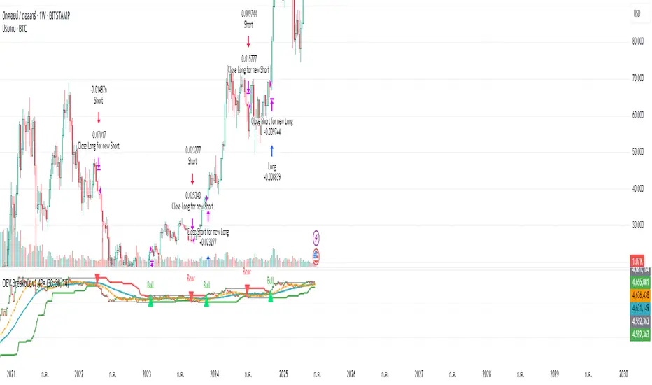
OBV ATR Strategy (OBV Breakout Channel) bas20230503ผมแก้ไขจาก OBV+SMA อันเดิม ของเดิม ดูที่เส้น SMA สองเส้นตัดกันมั่นห่วยแตกสำหรับที่ผมลองเทรดจริง และหลักการเบรค ได้แรงบันดาลใจ ATR จาก เทพคอย ที่ใช้กับราคา แต่นี้ใช้กับ OBV แทน
และผมใช้เจมินี้ เพื่อแก้ ให้ เป็น strategy เพื่อเช็คย้อนหลังได้ง่ายกว่าเดิม
หลักการง่ายคือถ้ามันขึ้น มันจะขึ้นเรื่อยๆ
เขียน แบบสุภาพ (น่าจะอ่านได้ง่ายกว่าผมเขียน)
สคริปต์นี้ได้รับการพัฒนาต่อยอดจากแนวคิด OBV+SMA Crossover แบบดั้งเดิม ซึ่งจากการทดสอบส่วนตัวพบว่าประสิทธิภาพยังไม่น่าพอใจ กลยุทธ์ใหม่นี้จึงเปลี่ยนมาใช้หลักการ "Breakout" ซึ่งได้รับแรงบันดาลใจมาจากการใช้ ATR สร้างกรอบของราคา แต่เราได้นำมาประยุกต์ใช้กับ On-Balance Volume (OBV) แทน นอกจากนี้ สคริปต์ได้ถูกแปลงเป็น Strategy เต็มรูปแบบ (โดยความช่วยเหลือจาก Gemini AI) เพื่อให้สามารถทดสอบย้อนหลัง (Backtest) และประเมินประสิทธิภาพได้อย่างแม่นยำ
หลักการของกลยุทธ์: กลยุทธ์นี้ทำงานบนแนวคิดโมเมนตัมที่ว่า "เมื่อแนวโน้มได้เกิดขึ้นแล้ว มีโอกาสที่มันจะดำเนินต่อไป" โดยจะมองหาการทะลุของพลังซื้อ-ขาย (OBV) ที่แข็งแกร่งเป็นพิเศษเป็นสัญญาณเข้าเทร
----
สคริปต์นี้เป็นกลยุทธ์ (Strategy) ที่ใช้ On-Balance Volume (OBV) ซึ่งเป็นอินดิเคเตอร์ที่วัดแรงซื้อและแรงขายสะสม แทนที่จะใช้การตัดกันของเส้นค่าเฉลี่ย (SMA Crossover) ที่เป็นแบบพื้นฐาน กลยุทธ์นี้จะมองหาการ "ทะลุ" (Breakout) ของพลัง OBV ออกจากกรอบสูงสุด-ต่ำสุดของตัวเองในรอบที่ผ่านมา
สัญญาณกระทิง (Bull Signal): เกิดขึ้นเมื่อพลังการซื้อ (OBV) แข็งแกร่งจนสามารถทะลุจุดสูงสุดของตัวเองในอดีตได้ บ่งบอกถึงโอกาสที่แนวโน้มจะเปลี่ยนเป็นขาขึ้น
สัญญาณหมี (Bear Signal): เกิดขึ้นเมื่อพลังการขาย (OBV) รุนแรงจนสามารถกดดันให้ OBV ทะลุจุดต่ำสุดของตัวเองในอดีตได้ บ่งบอกถึงโอกาสที่แนวโน้มจะเปลี่ยนเป็นขาลง
ส่วนประกอบบนกราฟ (Indicator Components)
เส้น OBV
เส้นหลัก ที่เปลี่ยนเขียวเป็นแดง เป็นทั้งแนวรับและแนวต้าน และ จุด stop loss
เส้นนี้คือหัวใจของอินดิเคเตอร์ ที่แสดงถึงพลังสะสมของ Volume
เมื่อเส้นเป็นสีเขียว (แนวรับ): จะปรากฏขึ้นเมื่อกลยุทธ์เข้าสู่ "โหมดกระทิง" เส้นนี้คือระดับต่ำสุดของ OBV ในอดีต และทำหน้าที่เป็นแนวรับไดนามิก
เมื่อเส้นกลายเป็นสีแดงสีแดง (แนวต้าน): จะปรากฏขึ้นเมื่อกลยุทธ์เข้าสู่ "โหมดหมี" เส้นนี้คือระดับสูงสุดของ OBV ในอดีต และทำหน้าที่เป็นแนวต้านไดนามิก
สัญลักษณ์สัญญาณ (Signal Markers):
Bull 🔼 (สามเหลี่ยมขึ้นสีเขียว): คือสัญญาณ "เข้าซื้อ" (Long) จะปรากฏขึ้น ณ จุดที่ OBV ทะลุขึ้นไปเหนือกรอบด้านบนเป็นครั้งแรก
Bear 🔽 (สามเหลี่ยมลงสีแดง): คือสัญญาณ "เข้าขาย" (Short) จะปรากฏขึ้น ณ จุดที่ OBV ทะลุลงไปต่ำกว่ากรอบด้านล่างเป็นครั้งแรก
วิธีการใช้งาน (How to Use)
เพิ่มสคริปต์นี้ลงบนกราฟราคาที่คุณสนใจ
ไปที่แท็บ "Strategy Tester" ด้านล่างของ TradingView เพื่อดูผลการทดสอบย้อนหลัง (Backtest) ของกลยุทธ์บนสินทรัพย์และไทม์เฟรมต่างๆ
ใช้สัญลักษณ์ "Bull" และ "Bear" เป็นตัวช่วยในการตัดสินใจเข้าเทรด
ข้อควรจำ: ไม่มีกลยุทธ์ใดที่สมบูรณ์แบบ 100% ควรใช้สคริปต์นี้ร่วมกับการวิเคราะห์ปัจจัยอื่นๆ เช่น โครงสร้างราคา, แนวรับ-แนวต้านของราคา และการบริหารความเสี่ยง (Risk Management) ของตัวคุณเองเสมอ
การตั้งค่า (Inputs)
SMA Length 1 / SMA Length 2: ใช้สำหรับพล็อตเส้นค่าเฉลี่ยของ OBV เพื่อดูเป็นภาพอ้างอิง ไม่มีผลต่อตรรกะการเข้า-ออกของ Strategy อันใหม่ แต่มันเป็นของเก่า ถ้าชอบ ก็ใช้ได้ เมื่อ SMA สองเส้นตัดกัน หรือตัดกับเส้น OBV
High/Low Lookback Length: (ค่าพื้นฐาน30/แก้ตรงนี้ให้เหมาะสมกับ coin หรือหุ้น ตามความผันผวน ) คือระยะเวลาที่ใช้ในการคำนวณกรอบสูงสุด-ต่ำสุดของ OBV
ค่าน้อย: ทำให้กรอบแคบลง สัญญาณจะเกิดไวและบ่อยขึ้น แต่อาจมีสัญญาณหลอก (False Signal) เยอะขึ้น
ค่ามาก: ทำให้กรอบกว้างขึ้น สัญญาณจะเกิดช้าลงและน้อยลง แต่มีแนวโน้มที่จะเป็นสัญญาณที่แข็งแกร่งกว่า
แน่นอนครับ นี่คือคำแปลฉบับภาษาอังกฤษที่สรุปใจความสำคัญ กระชับ และสุภาพ เหมาะสำหรับนำไปใช้ในคำอธิบายสคริปต์ (Description) ของ TradingView ครับ
---Translate to English---
OBV Breakout Channel Strategy
This script is an evolution of a traditional OBV+SMA Crossover concept. Through personal testing, the original crossover method was found to have unsatisfactory performance. This new strategy, therefore, uses a "Breakout" principle. The inspiration comes from using ATR to create price channels, but this concept has been adapted and applied to On-Balance Volume (OBV) instead.
Furthermore, the script has been converted into a full Strategy (with assistance from Gemini AI) to enable precise backtesting and performance evaluation.
The strategy's core principle is momentum-based: "once a trend is established, it is likely to continue." It seeks to enter trades on exceptionally strong breakouts of buying or selling pressure as measured by OBV.
Core Concept
This is a Strategy that uses On-Balance Volume (OBV), an indicator that measures cumulative buying and selling pressure. Instead of relying on a basic Simple Moving Average (SMA) Crossover, this strategy identifies a "Breakout" of the OBV from its own highest-high and lowest-low channel over a recent period.
Bull Signal: Occurs when the buying pressure (OBV) is strong enough to break above its own recent highest high, indicating a potential shift to an upward trend.
Bear Signal: Occurs when the selling pressure (OBV) is intense enough to push the OBV below its own recent lowest low, indicating a potential shift to a downward trend.
On-Screen Components
1. OBV Line
This is the main indicator line, representing the cumulative volume. Its color changes to green when OBV is rising and red when it is falling.
2. Dynamic Support & Resistance Line
This is the thick Green or Red line that appears based on the strategy's current "mode." This line serves as a dynamic support/resistance level and can be used as a reference for stop-loss placement.
Green Line (Support): Appears when the strategy enters "Bull Mode." This line represents the lowest low of the OBV in the recent past and acts as dynamic support.
Red Line (Resistance): Appears when the strategy enters "Bear Mode." This line represents the highest high of the OBV in the recent past and acts as dynamic resistance.
3. Signal Markers
Bull 🔼 (Green Up Triangle): This is the "Long Entry" signal. It appears at the moment the OBV first breaks out above its high-low channel.
Bear 🔽 (Red Down Triangle): This is the "Short Entry" signal. It appears at the moment the OBV first breaks down below its high-low channel.
How to Use
Add this script to the price chart of your choice.
Navigate to the "Strategy Tester" panel at the bottom of TradingView to view the backtesting results for the strategy on different assets and timeframes.
Use the "Bull" and "Bear" signals as aids in your trading decisions.
Disclaimer: No strategy is 100% perfect. This script should always be used in conjunction with other forms of analysis, such as price structure, key price-based support/resistance levels, and your own personal risk management rules.
Inputs
SMA Length 1 / SMA Length 2: These are used to plot moving averages on the OBV for visual reference. They are part of the legacy logic and do not affect the new breakout strategy. However, they are kept for traders who may wish to observe their crossovers for additional confirmation.
High/Low Lookback Length: (Most Important Setting) This determines the period used to calculate the highest-high and lowest-low OBV channel. (Default is 30; adjust this to suit the asset's volatility).
A smaller value: Creates a narrower channel, leading to more frequent and faster signals, but potentially more false signals.
A larger value: Creates a wider channel, leading to fewer and slower signals, which are likely to be more significant.
Cerca negli script per "the strat"
Strategic LevelsIntroduction
The Strategic Levels indicator plots key high and low price levels for monthly, weekly, daily, and Monday (current week) timeframes. It draws horizontal lines with consolidated labels to highlight significant support and resistance zones.
How to use it ?
Identify critical price levels for trade entries, exits, and risk management.
These prices levels (monthly, weekly, daily open/close) are significant inflection points during short term price movements.
Perfect for swing traders, day traders, or anyone using support/resistance strategies.
Best used for trades lasting no more than a few days.

Timeshifter Triple Timeframe Strategy w/ SessionsOverview
The "Enhanced Timeshifter Triple Timeframe Strategy with Session Filtering" is a sophisticated trading strategy designed for the TradingView platform. It integrates multiple technical indicators across three different timeframes and allows traders to customize their trading Sessions. This strategy is ideal for traders who wish to leverage multi-timeframe analysis and session-based trading to enhance their trading decisions.
Features
Multi-Timeframe Analysis and direction:
Higher Timeframe: Set to a daily timeframe by default, providing a broader view of market trends.
Trading Timeframe: Automatically set to the current chart timeframe, ensuring alignment with the trader's primary analysis period.
Lower Timeframe: Set to a 15-minute timeframe by default, offering a granular view for precise entry and exit points.
Indicator Selection:
RMI (Relative Momentum Index): Combines RSI and MFI to gauge market momentum.
TWAP (Time Weighted Average Price): Provides an average price over a specified period, useful for identifying trends.
TEMA (Triple Exponential Moving Average): Reduces lag and smooths price data for trend identification.
DEMA (Double Exponential Moving Average): Similar to TEMA, it reduces lag and provides a smoother trend line.
MA (Moving Average): A simple moving average for basic trend analysis.
MFI (Money Flow Index): Measures the flow of money into and out of a security, useful for identifying overbought or oversold conditions.
VWMA (Volume Weighted Moving Average): Incorporates volume data into the moving average calculation.
PSAR (Parabolic SAR): Identifies potential reversals in price movement.
Session Filtering:
London Session: Trade during the London market hours (0800-1700 GMT+1).
New York Session: Trade during the New York market hours (0800-1700 GMT-5).
Tokyo Session: Trade during the Tokyo market hours (0900-1800 GMT+9).
Users can select one or multiple sessions to align trading with specific market hours.
Trade Direction:
Long: Only long trades are permitted.
Short: Only short trades are permitted.
Both: Both long and short trades are permitted, providing flexibility based on market conditions.
ADX Confirmation:
ADX (Average Directional Index): An optional filter to confirm the strength of a trend before entering a trade.
How to Use the Script
Setup:
Add the script to your TradingView chart.
Customize the input parameters according to your trading preferences and strategy requirements.
Indicator Selection:
Choose the primary indicator you wish to use for generating trading signals from the dropdown menu.
Enable or disable the ADX confirmation based on your preference for trend strength analysis.
Session Filtering:
Select the trading sessions you wish to trade in. You can choose one or multiple Sessions based on your trading strategy and market focus.
Trade Direction:
Set your preferred trade direction (Long, Short, or Both) to align with your market outlook and risk tolerance. You can use this feature to gauge the market and understand the possible directions.
Tips for Profitable and Safe Trading:
Recommended Timeframes Combination:
LT: 1m , CT: 5m, HT: 1H
LT: 1-5m , CT: 15m, HT: 4H
LT: 5-15m , CT: 4H, HT: 1W
Backtesting:
Always backtest the strategy on historical data to understand its performance under various market conditions.
Adjust the parameters based on backtesting results to optimize the strategy for your specific trading style.
Risk Management:
Use appropriate risk management techniques, such as setting stop-loss and take-profit levels, to protect your capital.
Avoid over-leveraging and ensure that you are trading within your risk tolerance.
Market Analysis:
Combine the script with other forms of market analysis, such as fundamental analysis or market sentiment, to make well-rounded trading decisions.
Stay informed about major economic events and news that could impact market volatility and trading sessions.
Continuous Monitoring:
Regularly monitor the strategy's performance and make adjustments as necessary.
Keep an eye on the results and settings for real-time statistics and ensure that the strategy aligns with current market conditions.
Education and Practice:
Continuously educate yourself on trading strategies and market dynamics.
Practice using the strategy in a demo account before applying it to live trading to gain confidence and understanding.

Inside Bar Detector - 15min
🔍 What is an Inside Bar?
An **Inside Bar** is a candle that forms **entirely within the high and low of the previous candle**. It represents **consolidation**, **indecision**, or **potential reversal**, and is a key signal in The Strat trading method.
🔧 What the Script Does:
1. **Timeframe Restriction**:
* The script activates **only on the 15-minute timeframe**, avoiding clutter on other timeframes.
2. **Inside Bar Logic**:
* It checks whether the **current bar’s high is lower than the previous bar’s high**, **AND** the **current bar’s low is higher than the previous bar’s low**.
* If both conditions are true, it confirms an Inside Bar.
3. **Visual Display**:
* When an Inside Bar is detected, the script **plots a yellow label ("1") above the bar**.
* The label represents the Strat 1-bar and helps you easily spot potential setups.
🎯 Use Case:
* Ideal for **Strat traders**, **price action analysts**, or **any trader** looking for breakout or reversal opportunities.
* Common setups include **1-2**, **1-3**, or **double inside bar** breakouts.

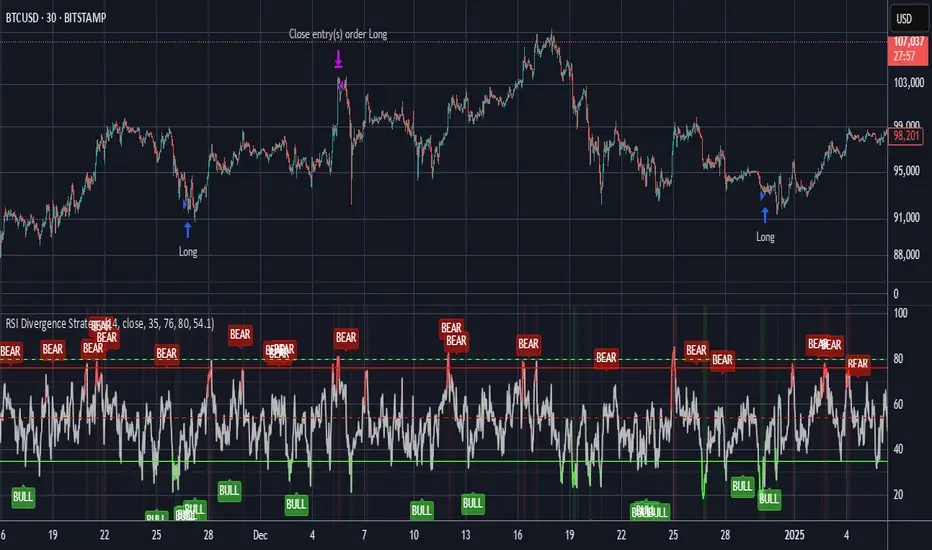
RSI Divergence StrategyOverview
The RSI Divergence Strategy Indicator is a trading tool that uses the RSI and divergences created to generate high-probability buy and sell signals.
I have provided the best formula of numbers to use for BTC on a 30 minute timeframe.
You can change where on RSI you enter and exit both long or short trades. This way you can experiment on different tokens using different entry/exit points. Can use on multiple timeframes.
This strategy is designed to open and close long or short trades based on the levels you provide it. You can then check on the RSI where the best levels are for each token you want to trade and amend it as required to generate a profitable strategy.
How It Works
The RSI Divergence Strategy Indicator uses bear and bull divergences in conjuction with a level you have input on the RSI.
RSI for Overbought/Oversold:
• Input variables for entry and exit levels and when the entry levels combine with a bear or bull divergence signal, a trade is alerted.
RSI Divergence:
• Buy and sell signals are confirmed when the RSI creates bearish or bullish divergences and these divergences are in the same area as your levels you input for entry to short or long.
After 7 years of experience and testing I have calculated the exact numbers required and produced a formula to calculate the exact input variables for a 30 minute Bitcoin chart.
Key Features
1️⃣ Divergence Identification – Ensures trades are taken only when a bull or bear divergence has formed.
2️⃣ Overbought/Oversold Input Filtering – Set up your own variables on the RSI for different markets after identifying patterns on the RSI in relation to a bearish or bullish divergence.
3️⃣ Works on any chart – Suitable for all markets and timeframes once you input the correct variables for entry and exit levels.
How to Use
🟢 Basic Trading:
• Use on any timeframe.
• Enter trade only when alert has fired off. Close when it says to exit.
• Change entry and exit levels in the properties of the strategy indicator.
• Make entry and exit levels coincide with bearish or bullish divergences on the RSI.
Check the strategy tester to see backtesting so you know if the indicator is profitable or not for that market and timeframe as each crypto token is different and so is the timeframe you choose.
📢 Webhook Automation:
• Set up TradingView Alerts to auto-execute trades via Webhook-compatible platforms.
Key additions for divergence visualization:
Divergence Arrows:
Bullish divergence: Green label with white 'bull ' text
Bearish divergence: Red label with white 'bear' text
Positioned at the pivot point
Divergence Lines:
Connects consecutive RSI pivot points
Automatically drawn between consecutive pivot points
Enhanced RSI Coloring:
Overbought zone: Red
Oversold zone: Green
Neutral zone: Gray
The visualization helps you instantly spot:
Where divergences are forming on the RSI
The pattern of higher lows (bullish) or lower highs (bearish)
Contextual coloring of RSI relative to standard levels
All divergence markers appear at the correct historical pivot points, making it easy to visually confirm divergence patterns as they develop.
Strategy levels and background zones also shown to help visual look.
Why This Combination?
This indicator is just a simple RSI tool.
It is designed to filter out weak trades and only execute trades that have:
✅ RSI Divergence
✅ Overbought or Oversold Conditions
It does not calculate downtrends or bear markets so care is recommended taking long trades during these times.
Why It’s Worth Using?
📈 Open Source – Free to use and learn from.
📉 Long or Short Term Trading Style – Entry/Exit parameters options are designed for both short or long term trades allowing you to experiment until you find a profitable strategy for that market you want to trade.
📢 Seamless Webhook Automation – Execute trades automatically with TradingView alerts.
💲 Ready to trade smarter?
✅ Add the RSI Divergence Strategy Indicator to your TradingView chart.
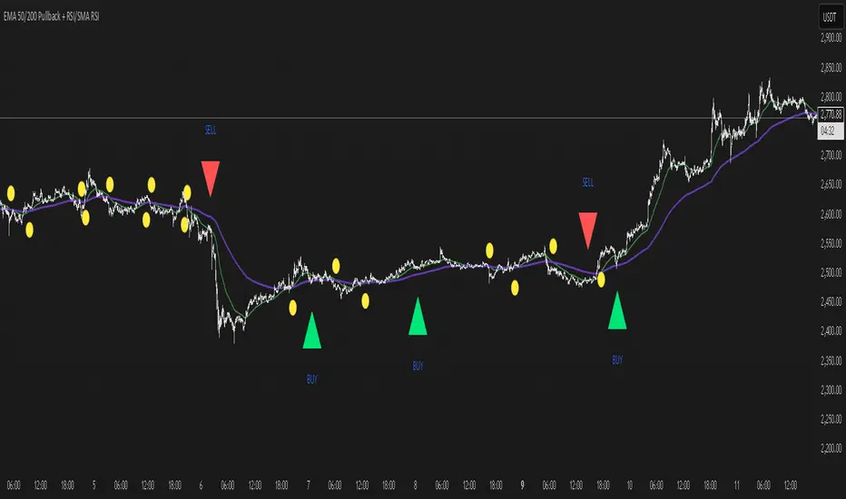
EMA 50/200 Pullback + RSI/SMA RSI
Strategy Description: EMA 50/200 Pullback + RSI/SMA RSI
1. Trend Identification with EMA:
Uses two Exponential Moving Averages (EMA): a fast EMA (default 50) and a slow EMA (default 200).
When the fast EMA crosses above the slow EMA (bullish crossover), an uptrend is identified.
When the fast EMA crosses below the slow EMA (bearish crossover), a downtrend is identified.
The lengths of both EMAs are fully customizable.
2. EMA Distance Condition:
Signals are only valid when the absolute percentage distance between the two EMAs is within a user-defined range (default: 0.4% to 1%).
This helps filter out weak signals when the EMAs are too close or too far apart.
3. Pullback Condition:
After a new trend is detected (EMA crossover), the strategy waits for the price to pull back to touch or cross the fast EMA (EMA 50).
This ensures entries are not taken immediately at the crossover, but after a retracement to a dynamic support/resistance area.
4. RSI Confirmation:
Uses the RSI indicator (default 14) and its Simple Moving Average (SMA RSI, default 14).
Buy signal: RSI crosses above its SMA.
Sell signal: RSI crosses below its SMA.
Both RSI and SMA RSI lengths are fully customizable.
5. Entry Rules:
The indicator only gives the first buy/sell signal after each EMA crossover (start of a new trend), and will not repeat signals until the next EMA crossover.
Buy signal:
Fast EMA crosses above slow EMA
EMA distance is within the valid range
Price pulls back to the fast EMA
RSI crosses above its SMA
Sell signal:
Fast EMA crosses below slow EMA
EMA distance is within the valid range
Price pulls back to the fast EMA
RSI crosses below its SMA
6. Customization:
All parameters (EMA lengths, RSI length, SMA RSI length, EMA distance range) can be adjusted in the indicator’s settings.
Note:
This is a signal indicator, not a complete trading strategy. For real trading, always combine with risk management and additional confirmations.
Zero Lag MACD + Kijun-sen + EOM StrategyThis strategy offers a robust approach to identifying high-probability trading opportunities in the fast-paced cryptocurrency markets, particularly on lower timeframes (e.g., 5-minute). It leverages the synergistic power of three distinct indicators to confirm entries, ensuring a disciplined approach to risk management.
Key Components:
Zero Lag MACD Enhanced Version 1.2: This core momentum indicator is used to identify precise shifts in trend and momentum, offering reduced lag compared to traditional MACD. Entry signals are filtered based on the histogram's position (below for buys, above for sells) to enhance signal reliability.
Kijun-sen (Ichimoku Cloud): Acting as a dynamic support/resistance and trend filter, the Kijun-sen line confirms the prevailing market direction. Long entries are confirmed when price is above Kijun-sen, and short entries when price is below.
Ease of Movement (EoM): This volume-based oscillator provides crucial confirmation of price movements by measuring the ease with which price changes. Positive EoM confirms buying pressure, while negative confirms selling pressure, adding an essential layer of validation to trade setups.
How it Works:
The strategy generates entry signals only when all three indicators align simultaneously:
For Long Entries: A Zero Lag MACD buy signal (crossover below histogram) must coincide with price trading above the Kijun-sen, and the Ease of Movement indicator being above its zero line.
For Short Entries: A Zero Lag MACD sell signal (crossover above histogram) must coincide with price trading below the Kijun-sen, and the Ease of Movement indicator being below its zero line.
Entries are executed at the open of the candle immediately following the signal confirmation.
Risk Management:
Disciplined risk management is paramount to this strategy:
Dynamic Stop-Loss: An Average True Range (ATR) based stop-loss is implemented, set at 2.5 times the current ATR. This adapts the stop-loss distance to market volatility, ensuring sensible risk sizing.
Fixed Take-Profit: A consistent Risk-to-Reward (R:R) ratio of 1:1.2 is applied for all trades, promoting stable profit realization.
Customization & Optimization:
The strategy is built with fully customizable input parameters for each indicator (MACD lengths, Kijun-sen period, ATR period, ATR multiplier, and Risk-to-Reward ratio). This allows users to fine-tune the strategy for different assets, timeframes, and market conditions, facilitating robust backtesting and optimization.
Disclaimer: Trading involves substantial risk and is not suitable for all investors. Past performance is not indicative of future results. This strategy is provided for educational and informational purposes only. Always use proper risk management and conduct your own due diligence.

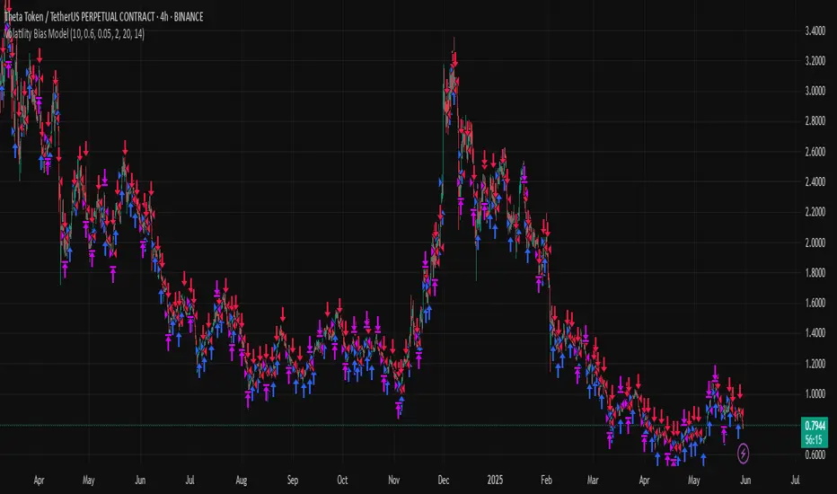
Volatility Bias ModelVolatility Bias Model
Overview
Volatility Bias Model is a purely mathematical, non-indicator-based trading system that detects directional probability shifts during high volatility market phases. Rather than relying on classic tools like RSI or moving averages, this strategy uses raw price behavior and clustering logic to determine potential breakout direction based on recent market bias.
How It Works
Over a defined lookback window (default 10 bars), the strategy counts how many candles closed in the same direction (i.e., bullish or bearish).
Simultaneously, it calculates the price range during that window.
If volatility is above a minimum threshold and a clear directional bias is detected (e.g., >60% of closes are bullish), a trade is opened in the direction of that bias.
This approach assumes that when high volatility is coupled with directional closing consistency, the market is probabilistically more likely to continue in that direction.
ATR-based stop-loss and take-profit levels are applied, and trades auto-exit after 20 bars if targets are not hit.
Key Features
- 100% non-indicator-based logic
- Statistically-driven directional bias detection
- Works across all timeframes (1H, 4H, 1D)
- ATR-based risk management
- No pyramiding, slippage and commissions included
- Compatible with real-world backtesting conditions
Realism & Assumptions
To make this strategy more aligned with actual trading environments, it includes 0.05% commission per trade and a 1-point slippage on every entry and exit.
Additionally, position sizing is set at 10% of a $10,000 starting capital, and no pyramiding is allowed.
These assumptions help avoid unrealistic backtest results and make the performance metrics more representative of live conditions.
Parameter Explanation
Bias Window (10 bars): Number of past candles used to evaluate directional closings
Bias Threshold (0.60): Required ratio of same-direction candles to consider a bias valid
Minimum Range (1.5%): Ensures the market is volatile enough to avoid noise
ATR Length (14): Used to dynamically define stop-loss and target zones
Risk-Reward Ratio (2.0): Take-profit is set at twice the stop-loss distance
Max Holding Bars (20): Trades are closed automatically after 20 bars to prevent stagnation
Originality Note
Unlike common strategies based on oscillators or moving averages, this script is built on pure statistical inference. It models the market as a probabilistic process and identifies directional intent based on historical closing behavior, filtered by volatility. This makes it a non-linear, adaptive model grounded in real-world price structure — not traditional technical indicators.
Disclaimer
This strategy is for educational and experimental purposes only. It does not constitute financial advice. Always perform your own analysis and test thoroughly before applying with real capital.
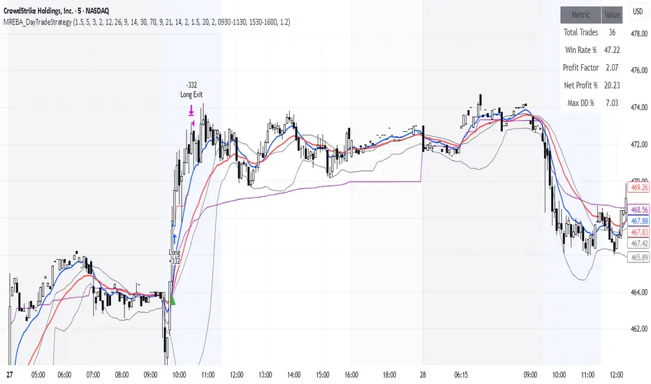
MACD + RSI + EMA + BB + ATR Day Trading StrategyEntry Conditions and Signals
The strategy implements a multi-layered filtering approach to entry conditions, requiring alignment across technical indicators, timeframes, and market conditions .
Long Entry Requirements
Trend Filter: Fast EMA (9) must be above Slow EMA (21), price must be above Fast EMA, and higher timeframe must confirm uptrend
MACD Signal: MACD line crosses above signal line, indicating increasing bullish momentum
RSI Condition: RSI below 70 (not overbought) but above 40 (showing momentum)
Volume & Volatility: Current volume exceeds 1.2x 20-period average and ATR shows sufficient market movement
Time Filter: Trading occurs during optimal hours (9:30-11:30 AM ET) when market volatility is typically highest
Exit Strategies
The strategy employs multiple exit mechanisms to adapt to changing market conditions and protect profits :
Stop Loss Management
Initial Stop: Placed at 2.0x ATR from entry price, adapting to current market volatility
Trailing Stop: 1.5x ATR trailing stop that moves up (for longs) or down (for shorts) as price moves favorably
Time-Based Exits: All positions closed by end of trading day (4:00 PM ET) to avoid overnight risk
Best Practices for Implementation
Settings
Chart Setup: 5-minute timeframe for execution with 15-minute chart for trend confirmation
Session Times: Focus on 9:30-11:30 AM ET trading for highest volatility and opportunity
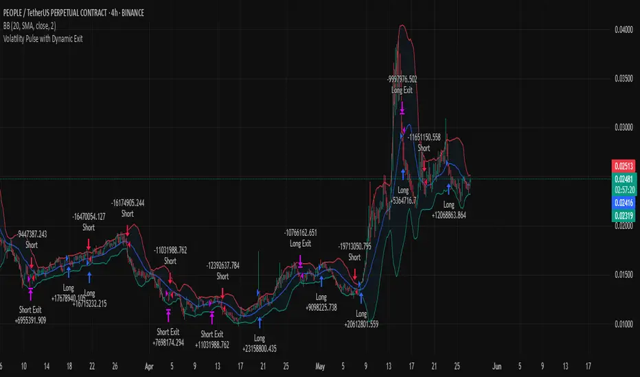
Volatility Pulse with Dynamic ExitVolatility Pulse with Dynamic Exit
Overview
This strategy, Volatility Pulse with Dynamic Exit, is designed to capture impulsive price moves following volatility expansions, while ensuring risk is managed dynamically. It avoids trades during low-volatility periods and uses momentum confirmation to enter positions. Additionally, it features a time-based forced exit system to limit overexposure.
How It Works
A position is opened when the current ATR (Average True Range) significantly exceeds its 20-period average, signaling a volatility expansion.
To confirm the move is directional and not random noise, the strategy checks for momentum: the close must be above/below the close of 20 bars ago.
Low volatility zones are filtered out to avoid chop and poor trade entries.
Upon entry, a dynamic stop-loss is set at 1x ATR, while take-profit is set at 2x ATR, offering a 2:1 reward-to-risk ratio.
If the position remains open for more than 42 bars, it is forcefully closed, even if targets are not hit. This prevents long-lasting, stagnant trades.
Key Features
✅ Volatility-based breakout detection
✅ Momentum confirmation filter
✅ Dynamic stop-loss and take-profit based on real-time ATR
✅ Time-based forced exit (42 bars max holding)
✅ Low-volatility environment filter
✅ Realistic settings with 0.05% commission and slippage included
Parameters Explanation
ATR Length (14): Captures recent volatility over ~2 weeks (14 candles).
Momentum Lookback (20): Ensures meaningful price move confirmation.
Volatility Expansion Threshold (0.5x): Strategy activates only when ATR is at least 50% above its average.
Minimum ATR Filter (1.0x): Avoids entries in tight, compressed market ranges.
Max Holding (42 bars): Trades are closed after 42 bars if no exit signal is triggered.
Risk-Reward (2.0x): Aiming for 2x ATR as profit for every 1x ATR risk.
Originality Note
While volatility and momentum have been used separately in many strategies, this script combines both with a time-based dynamic exit system. This exit rule, combined with an ATR-based filter to exclude low-activity periods, gives the system a practical edge in real-world use. It avoids classic rehashes and integrates real trading constraints for better applicability.
Disclaimer
This is a research-focused trading strategy meant for backtesting and educational purposes. Always use proper risk management and perform due diligence before applying to real funds.
magic wand STSM"Magic Wand STSM" Strategy: Trend-Following with Dynamic Risk Management
Overview:
The "Magic Wand STSM" (Supertrend & SMA Momentum) is an automated trading strategy designed to identify and capitalize on sustained trends in the market. It combines a multi-timeframe Supertrend for trend direction and potential reversal signals, along with a 200-period Simple Moving Average (SMA) for overall market bias. A key feature of this strategy is its dynamic position sizing based on a user-defined risk percentage per trade, and a built-in daily and monthly profit/loss tracking system to manage overall exposure and prevent overtrading.
How it Works (Underlying Concepts):
Multi-Timeframe Trend Confirmation (Supertrend):
The strategy uses two Supertrend indicators: one on the current chart timeframe and another on a higher timeframe (e.g., if your chart is 5-minute, the higher timeframe Supertrend might be 15-minute).
Trend Identification: The Supertrend's direction output is crucial. A negative direction indicates a bearish trend (price below Supertrend), while a positive direction indicates a bullish trend (price above Supertrend).
Confirmation: A core principle is that trades are only considered when the Supertrend on both the current and the higher timeframe align in the same direction. This helps to filter out noise and focus on stronger, more confirmed trends. For example, for a long trade, both Supertrends must be indicating a bearish trend (price below Supertrend line, implying an uptrend context where price is expected to stay above/rebound from Supertrend). Similarly, for short trades, both must be indicating a bullish trend (price above Supertrend line, implying a downtrend context where price is expected to stay below/retest Supertrend).
Trend "Readiness": The strategy specifically looks for situations where the Supertrend has been stable for a few bars (checking barssince the last direction change).
Long-Term Market Bias (200 SMA):
A 200-period Simple Moving Average is plotted on the chart.
Filter: For long trades, the price must be above the 200 SMA, confirming an overall bullish bias. For short trades, the price must be below the 200 SMA, confirming an overall bearish bias. This acts as a macro filter, ensuring trades are taken in alignment with the broader market direction.
"Lowest/Highest Value" Pullback Entries:
The strategy employs custom functions (LowestValueAndBar, HighestValueAndBar) to identify specific price action within the recent trend:
For Long Entries: It looks for a "buy ready" condition where the price has found a recent lowest point within a specific number of bars since the Supertrend turned bearish (indicating an uptrend). This suggests a potential pullback or consolidation before continuation. The entry trigger is a close above the open of this identified lowest bar, and also above the current bar's open.
For Short Entries: It looks for a "sell ready" condition where the price has found a recent highest point within a specific number of bars since the Supertrend turned bullish (indicating a downtrend). This suggests a potential rally or consolidation before continuation downwards. The entry trigger is a close below the open of this identified highest bar, and also below the current bar's open.
Candle Confirmation: The strategy also incorporates a check on the candle type at the "lowest/highest value" bar (e.g., closevalue_b < openvalue_b for buy signals, meaning a bearish candle at the low, suggesting a potential reversal before a buy).
Risk Management and Position Sizing:
Dynamic Lot Sizing: The lotsvalue function calculates the appropriate position size based on your Your Equity input, the Risk to Reward ratio, and your risk percentage for your balance % input. This ensures that the capital risked per trade remains consistent as a percentage of your equity, regardless of the instrument's volatility or price. The stop loss distance is directly used in this calculation.
Fixed Risk Reward: All trades are entered with a predefined Risk to Reward ratio (default 2.0). This means for every unit of risk (stop loss distance), the target profit is rr times that distance.
Daily and Monthly Performance Monitoring:
The strategy tracks todaysWins, todaysLosses, and res (daily net result) in real-time.
A "daily profit target" is implemented (day_profit): If the daily net result is very favorable (e.g., res >= 4 with todaysLosses >= 2 or todaysWins + todaysLosses >= 8), the strategy may temporarily halt trading for the remainder of the session to "lock in" profits and prevent overtrading during volatile periods.
A "monthly stop-out" (monthly_trade) is implemented: If the lres (overall net result from all closed trades) falls below a certain threshold (e.g., -12), the strategy will stop trading for a set period (one week in this case) to protect capital during prolonged drawdowns.
Trade Execution:
Entry Triggers: Trades are entered when all buy/sell conditions (Supertrend alignment, SMA filter, "buy/sell situation" candle confirmation, and risk management checks) are met, and there are no open positions.
Stop Loss and Take Profit:
Stop Loss: The stop loss is dynamically placed at the upTrendValue for long trades and downTrendValue for short trades. These values are derived from the Supertrend indicator, which naturally adjusts to market volatility.
Take Profit: The take profit is calculated based on the entry price, the stop loss, and the Risk to Reward ratio (rr).
Position Locks: lock_long and lock_short variables prevent immediate re-entry into the same direction once a trade is initiated, or after a trend reversal based on Supertrend changes.
Visual Elements:
The 200 SMA is plotted in yellow.
Entry, Stop Loss, and Take Profit lines are plotted in white, red, and green respectively when a trade is active, with shaded areas between them to visually represent risk and reward.
Diamond shapes are plotted at the bottom of the chart (green for potential buy signals, red for potential sell signals) to visually indicate when the buy_sit or sell_sit conditions are met, along with other key filters.
A comprehensive trade statistics table is displayed on the chart, showing daily wins/losses, daily profit, total deals, and overall profit/loss.
A background color indicates the active trading session.
Ideal Usage:
This strategy is best applied to instruments with clear trends and sufficient liquidity. Users should carefully adjust the Your Equity, Risk to Reward, and risk percentage inputs to align with their individual risk tolerance and capital. Experimentation with different ATR Length and Factor values for the Supertrend might be beneficial depending on the asset and timeframe.

SMA Backtest Optimizer [Mr_Rakun]The SMA Backtest Optimizer is a powerful Pine Script tool designed to systematically analyze and compare various Simple Moving Average (SMA) periods to identify the most profitable configuration for trading strategies. This indicator tests multiple SMA periods (from 10 to 100) using a crossover strategy where buys occur when price crosses above the SMA and sells when price crosses below it.
Key Features:
Tests 10 different SMA periods to determine optimal settings
Calculates profit/loss based on a defined starting capital
Tracks total profit and number of trades for each period
Visually highlights the best performing SMA on your chart
Displays comprehensive results in an easy-to-read table
Labels the chart with key performance metrics
This code serves as a core framework that traders can customize for their specific needs. You can easily modify the strategy parameters, test different technical indicators, adjust capital settings, or implement more complex entry/exit rules. The optimization methodology can be applied to virtually any trading approach you wish to evaluate.
Feel free to adapt this framework to test your own trading ideas and discover which parameters work best in different market conditions.

CANX MA Crossover© CanxStixTrader
Moving average crossover systems measure drift in the market. They are great strategies for time-limited traders. KEEP IT SIMPLE
This strategy works both for buys and sells using the reaction line to guide your position against the reactions.
HOW TO USE THE INDICATOR
1) Choose your market and timeframe.
2) Choose the length.
3) Choose the multiplier.
4) Choose if the strategy is long-only or bidirectional (longs & shorts).
TIPS
The strategy works best in bullish markets as that is the primary direction that market such as stocks, indexes and metals like to move.
- Increase the multiplier to reduce whipsaws
- Increase the length to take fewer trades
- Decrease the length to take more trades
- Try a Long-Only strategy to see if that performs better.
The base set up when you load the indicator is for the 1 minute chart on gold. We found that it also works well on the US Indexes. For other markets you may need to change the length and multiplier to suit the market and back test its results.

EMA 10/20/50 Alignment Strategy### 📘 **Strategy Name**
**EMA 10/20/50 Trend Alignment Strategy**
---
### 📝 **Description (for Publishing)**
This strategy uses the alignment of Exponential Moving Averages (EMAs) to identify strong bullish trends. It enters a long position when the short-term EMA is above the mid-term EMA, which is above the long-term EMA — a classic sign of trend strength.
#### 🔹 Entry Criteria:
* **EMA10 > EMA20 > EMA50**: A bullish alignment that signals momentum in an upward direction.
* The strategy enters a **long position** when this alignment occurs.
#### 🔹 Exit Criteria:
* The long position is closed when the EMA alignment breaks (i.e., the trend weakens or reverses).
#### 🔹 Additional Features:
* Includes a **date range filter**, allowing you to backtest the strategy over a specific period.
* Uses **100% of available capital** for each trade (position size auto-scales with account balance).
* No short positions, stop loss, or take profit are applied — this is a trend-following strategy meant to ride bullish moves.
---
### ✅ Best For:
* Traders looking for a **simple, trend-based entry system**
* Testing price momentum strategies during specific market regimes
* Visualizing EMA stacking patterns in historical data

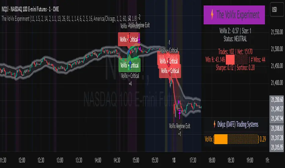
The VoVix Experiment The VoVix Experiment
The VoVix Experiment is a next-generation, regime-aware, volatility-adaptive trading strategy for futures, indices, and more. It combines a proprietary VoVix (volatility-of-volatility) anomaly detector with price structure clustering and critical point logic, only trading when multiple independent signals align. The system is designed for robustness, transparency, and real-world execution.
Logic:
VoVix Regime Engine: Detects pre-move volatility anomalies using a fast/slow ATR ratio, normalized by Z-score. Only trades when a true regime spike is detected, not just random volatility.
Cluster & Critical Point Filters: Price structure and volatility clustering must confirm the VoVix signal, reducing false positives and whipsaws.
Adaptive Sizing: Position size scales up for “super-spikes” and down for normal events, always within user-defined min/max.
Session Control: Trades only during user-defined hours and days, avoiding illiquid or high-risk periods.
Visuals: Aurora Flux Bands (From another Original of Mine (Options Flux Flow): glow and change color on signals, with a live dashboard, regime heatmap, and VoVix progression bar for instant insight.
Backtest Settings
Initial capital: $10,000
Commission: Conservative, realistic roundtrip cost:
15–20 per contract (including slippage per side) I set this to $25
Slippage: 3 ticks per trade
Symbol: CME_MINI:NQ1!
Timeframe: 15 min (but works on all timeframes)
Order size: Adaptive, 1–2 contracts
Session: 5:00–15:00 America/Chicago (default, fully adjustable)
Why these settings?
These settings are intentionally strict and realistic, reflecting the true costs and risks of live trading. The 10,000 account size is accessible for most retail traders. 25/contract including 3 ticks of slippage are on the high side for MNQ, ensuring the strategy is not curve-fit to perfect fills. If it works here, it will work in real conditions.
Forward Testing: (This is no guarantee. I've provided these results to show that executions perform as intended. Test were done on Tradovate)
ALL TRADES
Gross P/L: $12,907.50
# of Trades: 64
# of Contracts: 186
Avg. Trade Time: 1h 55min 52sec
Longest Trade Time: 55h 46min 53sec
% Profitable Trades: 59.38%
Expectancy: $201.68
Trade Fees & Comm.: $(330.95)
Total P/L: $12,576.55
Winning Trades: 59.38%
Breakeven Trades: 3.12%
Losing Trades: 37.50%
Link: www.dropbox.com
Inputs & Tooltips
VoVix Regime Execution: Enable/disable the core VoVix anomaly detector.
Volatility Clustering: Require price/volatility clusters to confirm VoVix signals.
Critical Point Detector: Require price to be at a statistically significant distance from the mean (regime break).
VoVix Fast ATR Length: Short ATR for fast volatility detection (lower = more sensitive).
VoVix Slow ATR Length: Long ATR for baseline regime (higher = more stable).
VoVix Z-Score Window: Lookback for Z-score normalization (higher = smoother, lower = more reactive).
VoVix Entry Z-Score: Minimum Z-score for a VoVix spike to trigger a trade.
VoVix Exit Z-Score: Z-score below which the regime is considered decayed (exit).
VoVix Local Max Window: Bars to check for local maximum in VoVix (higher = stricter).
VoVix Super-Spike Z-Score: Z-score for “super” regime events (scales up position size).
Min/Max Contracts: Adaptive position sizing range.
Session Start/End Hour: Only trade between these hours (exchange time).
Allow Weekend Trading: Enable/disable trading on weekends.
Session Timezone: Timezone for session filter (e.g., America/Chicago for CME).
Show Trade Labels: Show/hide entry/exit labels on chart.
Flux Glow Opacity: Opacity of Aurora Flux Bands (0–100).
Flux Band EMA Length: EMA period for band center.
Flux Band ATR Multiplier: Width of bands (higher = wider).
Compliance & Transparency
* No hidden logic, no repainting, no pyramiding.
* All signals, sizing, and exits are fully explained and visible.
* Backtest settings are stricter than most real accounts.
* All visuals are directly tied to the strategy logic.
* This is not a mashup or cosmetic overlay; every component is original and justified.
Disclaimer
Trading is risky. This script is for educational and research purposes only. Do not trade with money you cannot afford to lose. Past performance is not indicative of future results. Always test in simulation before live trading.
Proprietary Logic & Originality Statement
This script, “The VoVix Experiment,” is the result of original research and development. All core logic, algorithms, and visualizations—including the VoVix regime detection engine, adaptive execution, volatility/divergence bands, and dashboard—are proprietary and unique to this project.
1. VoVix Regime Logic
The concept of “volatility of volatility” (VoVix) is an original quant idea, not a standard indicator. The implementation here (fast/slow ATR ratio, Z-score normalization, local max logic, super-spike scaling) is custom and not found in public TradingView scripts.
2. Cluster & Critical Point Logic
Volatility clustering and “critical point” detection (using price distance from a rolling mean and standard deviation) are general quant concepts, but the way they are combined and filtered here is unique to this script. The specific logic for “clustered chop” and “critical point” is not a copy of any public indicator.
3. Adaptive Sizing
The adaptive sizing logic (scaling contracts based on regime strength) is custom and not a standard TradingView feature or public script.
4. Time Block/Session Control
The session filter is a common feature in many strategies, but the implementation here (with timezone and weekend control) is written from scratch.
5. Aurora Flux Bands (From another Original of Mine (Options Flux Flow)
The “glowing” bands are inspired by the idea of volatility bands (like Bollinger Bands or Keltner Channels), but the visual effect, color logic, and integration with regime signals are original to this script.
6. Dashboard, Watermark, and Metrics
The dashboard, real-time Sharpe/Sortino, and VoVix progression bar are all custom code, not copied from any public script.
What is “standard” or “common quant practice”?
Using ATR, EMA, and Z-score are standard quant tools, but the way they are combined, filtered, and visualized here is unique. The structure and logic of this script are original and not a mashup of public code.
This script is 100% original work. All logic, visuals, and execution are custom-coded for this project. No code or logic is directly copied from any public or private script.
Use with discipline. Trade your edge.
— Dskyz, for DAFE Trading Systems
REVELATIONS (VoVix - PoC) REVELATIONS (VoVix - POC): True Regime Detection Before the Move
Let’s not sugarcoat it: Most strategies on TradingView are recycled—RSI, MACD, OBV, CCI, Stochastics. They all lag. No matter how many overlays you stack, every one of these “standard” indicators fires after the move is underway. The retail crowd almost always gets in late. That’s never been enough for my team, for DAFE, or for anyone who’s traded enough to know the real edge vanishes by the time the masses react.
How is this different?
REVELATIONS (VoVix - POC) was engineered from raw principle, structured to detect pre-move regime change—before standard technicals even light up. We built, tested, and refined VoVix to answer one hard question:
What if you could see the spike before the trend?
Here’s what sets this system apart, line-by-line:
o True volatility-of-volatility mathematics: It’s not just "ATR of ATR" or noise smoothing. VoVix uses normalized, multi-timeframe v-vol spikes, instantly detecting orderbook stress and "outlier" market events—before the chart shows them as trends.
o Purist regime clustering: Every trade is enabled only during coordinated, multi-filter regime stress. No more signals in meaningless chop.
o Nonlinear entry logic: No trade is ever sent just for a “good enough” condition. Every entry fires only if every requirement is aligned—local extremes, super-spike threshold, regime index, higher timeframe, all must trigger in sync.
o Adaptive position size: Your contracts scale up with event strength. Tiny size during nominal moves, max leverage during true regime breaks—never guesswork, never static exposure.
o All exits governed by regime decay logic: Trades are closed not just on price targets but at the precise moment the market regime exhausts—the hardest part of systemic trading, now solved.
How this destroys the lag:
Standard indicators (RSI, MACD, OBV, CCI, and even most “momentum” overlays) simply tell you what already happened. VoVix triggers as price structure transitions—anyone running these generic scripts will trade behind the move while VoVix gets in as stress emerges. Real alpha comes from anticipation, not confirmation.
The visuals only show what matters:
Top right, you get a live, live quant dashboard—regime index, current position size, real-time performance (Sharpe, Sortino, win rate, and wins). Bottom right: a VoVix "engine bar" that adapts live with regime stress. Everything you see is a direct function of logic driving this edge—no cosmetics, no fake momentum.
Inputs/Signals—explained carefully for clarity:
o ATR Fast Length & ATR Slow Length:
These are the heart of VoVix’s regime sensing. Fast ATR reacts to sharp volatility; Slow ATR is stability baseline. Lower Fast = reacts to every twitch; higher Slow = requires more persistent, “real” regime shifts.
Tip: If you want more signals or faster markets, lower ATR Fast. To eliminate noise, raise ATR Slow.
o ATR StdDev Window: Smoothing for volatility-of-volatility normalization. Lower = more jumpy, higher = only the cleanest spikes trigger.
Tip: Shorten for “jumpy” assets, raise for indices/futures.
o Base Spike Threshold: Think of this as your “minimum event strength.” If the current move isn’t volatile enough (normalized), no signal.
Tip: Higher = only biggest moves matter. Lower for more signals but more potential noise.
o Super Spike Multiplier: The “are you sure?” test—entry only when the current spike is this multiple above local average.
Tip: Raise for ultra-selective/swing-trading; lower for more active style.
Regime & MultiTF:
o Regime Window (Bars):
How many bars to scan for regime cluster “events.” Short for turbo markets, long for big swings/trends only.
o Regime Event Count: Only trade when this many spikes occur within the Regime Window—filters for real stress, not isolated ticks.
Tip: Raise to only ever trade during true breakouts/crashes.
o Local Window for Extremes:
How many bars to check that a spike is a local max.
Tip: Raise to demand only true, “clearest” local regime events; lower for early triggers.
o HTF Confirm:
Higher timeframe regime confirmation (like 45m on an intraday chart). Ensures any event you act on is visible in the broader context.
Tip: Use higher timeframes for only major moves; lower for scalping or fast regimes.
Adaptive Sizing:
o Max Contracts (Adaptive): The largest size your system will ever scale to, even on extreme event.
Tip: Lower for small accounts/conservative risk; raise on big accounts or when you're willing to go big only on outlier events.
o Min Contracts (Adaptive): The “toe-in-the-water.” Smallest possible trade.
Tip: Set as low as your broker/exchange allows for safety, or higher if you want to always have meaningful skin in the game.
Trade Management:
o Stop %: Tightness of your stop-loss relative to entry. Lower for tighter/safer, higher for more breathing room at cost of greater drawdown.
o Take Profit %: How much you'll hold out for on a win. Lower = more scalps. Higher = only run with the best.
o Decay Exit Sensitivity Buffer: Regime index must dip this far below the trading threshold before you exit for “regime decay.”
Tip: 0 = exit as soon as stress fails, higher = exits only on stronger confirmation regime is over.
o Bars Decay Must Persist to Exit: How long must decay be present before system closes—set higher to avoid quick fades and whipsaws.
Backtest Settings
Initial capital: $10,000
Commission: Conservative, realistic roundtrip cost:
15–20 per contract (including slippage per side) I set this to $25
Slippage: 3 ticks per trade
Symbol: CME_MINI:NQ1!
Timeframe: 1 min (but works on all timeframes)
Order size: Adaptive, 1–3 contracts
No pyramiding, no hidden DCA
Why these settings?
These settings are intentionally strict and realistic, reflecting the true costs and risks of live trading. The 10,000 account size is accessible for most retail traders. 25/contract including 3 ticks of slippage are on the high side for NQ, ensuring the strategy is not curve-fit to perfect fills. If it works here, it will work in real conditions.
Tip: Set to 1 for instant regime exit; raise for extra confirmation (less whipsaw risk, exits held longer).
________________________________________
Bottom line: Tune the sensitivity, selectivity, and risk of REVELATIONS by these inputs. Raise thresholds and windows for only the best, most powerful signals (institutional style); lower for activity (scalpers, fast cryptos, signals in constant motion). Sizing is always adaptive—never static or martingale. Exits are always based on both price and regime health. Every input is there for your control, not to sell “complexity.” Use with discipline, and make it your own.
This strategy is not just a technical achievement: It’s a statement about trading smarter, not just more.
* I went back through the code to make sure no the strategy would not suffer from repainting, forward looking, or any frowned upon loopholes.
Disclaimer:
Trading is risky and carries the risk of substantial loss. Do not use funds you aren’t prepared to lose. This is for research and informational purposes only, not financial advice. Backtest, paper trade, and know your risk before going live. Past performance is not a guarantee of future results.
Expect more: We’ll keep pushing the standard, keep evolving the bar until “quant” actually means something in the public code space.
Use with clarity, use with discipline, and always trade your edge.
— Dskyz , for DAFE Trading Systems

Order Block with BoSHere’s a professional and concise description you can use for publishing your **TradingView script** titled **"Order Block with BoS"**:
---
### 📌 **Description for TradingView Publication:**
**"Order Block with Break of Structure (BoS)"** is a powerful price action-based indicator designed to identify potential reversal zones and momentum shifts using **Order Block** detection combined with **Break of Structure (BoS)** confirmation.
### 🔍 **Key Features:**
* **Order Block Detection**: Highlights bullish and bearish order blocks using precise candle structure logic.
* **Break of Structure (BoS)**: Confirms structural breaks above swing highs or below swing lows to validate potential trend continuation or reversal.
* **Dynamic ATR Filter**: Uses a 14-period ATR with dynamic thresholds to confirm significant moves, filtering out weak breakouts.
* **Visual Aids**:
* Color-coded **boxes** to mark detected Order Blocks.
* **Arrows** at BoS confirmation points when ATR confirms strong momentum.
* Optional **dashed BoS lines** to show where price broke structure.
### ⚙️ **Customizable Inputs**:
* `Swing Length`: Defines the sensitivity of swing high/low detection.
* `Show Break of Structure`: Toggle on/off BoS confirmation lines.
* `Candle Lookback`: Number of historical candles to consider.
This indicator is ideal for traders who incorporate **smart money concepts**, **market structure analysis**, or **institutional order flow** strategies.
---
Would you like me to help write the **strategy** version of this or translate the description into another language for international audiences?

Stochastic RSI with MTF TableShort Description of the Script
The provided Pine Script indicator, titled "Stochastic RSI with MTF Table," calculates and displays the Stochastic RSI for the current timeframe and multiple other timeframes (5m, 15m, 30m, 60m, 240m, and daily). The Stochastic RSI is a momentum indicator that blends the Relative Strength Index (RSI) and Stochastic Oscillator to identify overbought and oversold conditions, as well as potential trend reversals via K and D line crossovers.
Key features of the script include:
Inputs: Customizable parameters such as K smoothing (default 3), D smoothing (default 3), RSI length (default 14), Stochastic length (default 14), source price (default close), and overbought/oversold levels (default 80/20).
MTF Table: A table displays the Stochastic RSI status for each timeframe:
"OB" (overbought) if K > 80, "OS" (oversold) if K < 20, or "N" (neutral) otherwise.
Crossovers: "K↑D" for bullish (K crosses above D) and "K↓D" for bearish (K crosses below D).
Visualization: Plots the K and D lines for the current timeframe, with horizontal lines at 80 (overbought), 50 (middle), and 20 (oversold), plus a background fill for clarity.
Table Position: Configurable to appear in one of four chart corners (default: top-right).
This indicator helps traders assess momentum across multiple timeframes simultaneously, aiding in the identification of trend strength and potential entry/exit points.
Trading Strategy with 50EMA and 200EMA for Highest Winning Rate
To create a strategy with the best probability of a high winning rate using the Stochastic RSI MTF indicator alongside the 50-period Exponential Moving Average (50EMA) and 200-period Exponential Moving Average (200EMA), we can combine trend identification with momentum-based entry timing. The 50EMA and 200EMA are widely used to determine medium- and long-term trends, while the Stochastic RSI MTF table provides multi-timeframe momentum signals. Here’s the strategy:
1. Determine the Overall Trend
Bullish Trend: The 50EMA is above the 200EMA on the current timeframe (e.g., daily or 60m chart). This suggests an uptrend, often associated with a "Golden Cross."
Bearish Trend: The 50EMA is below the 200EMA on the current timeframe. This indicates a downtrend, often linked to a "Death Cross."
Implementation: Plot the 50EMA and 200EMA on your chart and visually confirm their relative positions.
2. Identify Entry Signals Using the Stochastic RSI MTF Table
In a Bullish Trend (50EMA > 200EMA):
Look for timeframes in the MTF table showing:
Oversold (OS): K < 20, indicating a potential pullback in the uptrend where price may rebound.
Bullish Crossover (K↑D): K crosses above D, signaling rising momentum and a potential entry point.
Example: If the 60m and 240m timeframes show "OS" or "K↑D," this could be a buy signal.
In a Bearish Trend (50EMA < 200EMA):
Look for timeframes in the MTF table showing:
Overbought (OB): K > 80, suggesting a rally in the downtrend where price may reverse downward.
Bearish Crossover (K↓D): K crosses below D, indicating declining momentum and a potential short entry.
Example: If the 30m and daily timeframes show "OB" or "K↓D," this could be a sell/short signal.
Current Timeframe Check: Use the plotted K and D lines on your trading timeframe for precise entry timing (e.g., confirm a K↑D crossover on a 60m chart for a long trade).
3. Confirm Signals Across Multiple Timeframes
Strengthen the Signal: A higher winning rate is more likely when multiple timeframes align with the trend and signal. For instance:
Bullish trend + "OS" or "K↑D" on 60m, 240m, and daily = strong buy signal.
Bearish trend + "OB" or "K↓D" on 15m, 60m, and 240m = strong sell signal.
Prioritize Higher Timeframes: Signals from the 240m or daily timeframe carry more weight due to their indication of broader trends, increasing reliability.
4. Set Stop-Loss and Take-Profit Levels
Long Trades (Bullish):
Stop-Loss: Place below the most recent swing low or below the 50EMA, whichever is closer, to protect against trend reversals.
Take-Profit: Target a key resistance level or use a risk-reward ratio (e.g., 2:1 or 3:1) based on the stop-loss distance.
Short Trades (Bearish):
Stop-Loss: Place above the most recent swing high or above the 50EMA, whichever is closer.
Take-Profit: Target a key support level or apply a similar risk-reward ratio.
Trailing Stop Option: As the trend progresses, trail the stop below the 50EMA (for longs) or above it (for shorts) to lock in profits.
5. Risk Management
Position Sizing: Risk no more than 1-2% of your trading capital per trade to minimize losses from false signals.
Volatility Consideration: Adjust stop-loss distances and position sizes based on the asset’s volatility (e.g., wider stops for volatile stocks or crypto).
Avoid Overtrading: Wait for clear alignment between the EMA trend and MTF signals to avoid low-probability setups.
Example Scenario
Chart: 60-minute timeframe.
Trend: 50EMA > 200EMA (bullish).
MTF Table: 60m shows "OS," 240m shows "K↑D," and daily is "N."
Action: Enter a long position when the 60m K line crosses above D, confirming the table signal.
Stop-Loss: Below the recent 60m swing low (e.g., 2% below entry).
Take-Profit: At the next resistance level or a 3:1 reward-to-risk ratio.
Outcome: High probability of success due to trend alignment and multi-timeframe confirmation.
Why This Strategy Works
Trend Following: Trading in the direction of the 50EMA/200EMA trend reduces the risk of fighting the market’s momentum.
Momentum Timing: The Stochastic RSI MTF table pinpoints pullbacks or reversals within the trend, improving entry timing.
Multi-Timeframe Confirmation: Alignment across timeframes filters out noise, increasing the win rate.
Risk Control: Defined stop-loss and position sizing protect against inevitable losses.
Caveats
No strategy guarantees a 100% win rate; false signals can occur, especially in choppy markets.
Test this strategy on historical data or a demo account to verify its effectiveness for your asset and timeframe.
This approach leverages the strengths of both trend-following (EMA) and momentum (Stochastic RSI) tools, aiming for a high-probability, disciplined trading system.

UTSStrategyHelperLibrary "UTSStrategyHelper"
TODO: add library description here
stopLossPrice(sig, atr, factor, isLong)
Calculates the stop loss price using a distance determined by ATR multiplied by a factor. Example for Long trade SL: PRICE - (ATR * factor).
Parameters:
sig (float)
atr (float) : (float): The value of the atr.
factor (float)
isLong (bool) : (bool): The current trade direction.
Returns: (bool): A boolean value.
takeProfitPrice(sig, atr, factor, isLong)
Calculates the take profit price using a distance determined by ATR multiplied by a factor. Example for Long trade TP: PRICE + (ATR * factor). When take profit price is reached usually 50 % of the position is closed and the other 50 % get a trailing stop assigned.
Parameters:
sig (float)
atr (float) : (float): The value of the atr.
factor (float)
isLong (bool) : (bool): The current trade direction.
Returns: (bool): A boolean value.
trailingStopPrice(initialStopPrice, atr, factor, priceSource, isLong)
Calculates a trailing stop price using a distance determined by ATR multiplied by a factor. It takes an initial price and follows the price closely if it changes in a favourable way.
Parameters:
initialStopPrice (float) : (float): The initial stop price which, for consistency also should be ATR * factor behind price: e.g. Long trade: PRICE - (ATR * factor)
atr (float) : (float): The value of the atr. Ideally the ATR value at trade open is taken and used for subsequent calculations.
factor (float)
priceSource (float) : (float): The current price.
isLong (bool) : (bool): The current trade direction.
Returns: (bool): A boolean value.
hasGreaterPositionSize(positionSize)
Determines if the strategy's position size has grown since the last bar.
Parameters:
positionSize (float) : (float): The size of the position.
Returns: (bool): A boolean value.
hasSmallerPositionSize(positionSize)
Determines if the strategy's position size has decreased since the last bar.
Parameters:
positionSize (float) : (float): The size of the position.
Returns: (bool): A boolean value.
hasUnchangedPositionSize(positionSize)
Determines if the strategy's position size has changed since the last bar.
Parameters:
positionSize (float) : (float): The size of the position.
Returns: (bool): A boolean value.
exporthasLongPosition(positionSize)
Determines if the strategy has an open long position.
Parameters:
positionSize (float) : (float): The size of the position.
Returns: (bool): A boolean value.
hasShortPosition(positionSize)
Determines if the strategy has an open short position.
Parameters:
positionSize (float) : (float): The size of the position.
Returns: (bool): A boolean value.
hasAnyPosition(positionSize)
Determines if the strategy has any open position, regardless of short or long.
Parameters:
positionSize (float) : (float): The size of the position.
Returns: (bool): A boolean value.
hasSignal(value)
Determines if the given argument contains a valid value (means not 'na').
Parameters:
value (float) : (float): The actual value.
Returns: (bool): A boolean value.

Best SMA FinderThis script, Best SMA Finder, is a tool designed to identify the most robust simple moving average (SMA) length for a given chart, based on historical backtest performance. It evaluates hundreds of SMA values (from 10 to 1000) and selects the one that provides the best balance between profitability, consistency, and trade frequency.
What it does:
The script performs individual backtests for each SMA length using either "Long Only" or "Buy & Sell" logic, as selected by the user. For each tested SMA, it computes:
- Total number of trades
- Profit Factor (total profits / total losses)
- Win Rate
- A composite Robustness Score, which integrates Profit Factor, number of trades (log-scaled), and win rate.
Only SMA configurations that meet the user-defined minimum trade count are considered valid. Among all valid candidates, the script selects the SMA length with the highest robustness score and plots it on the chart.
How to use it:
- Choose the strategy type: "Long Only" or "Buy & Sell"
- Set the minimum trade count to filter out statistically irrelevant results
- Enable or disable the summary stats table (default: enabled)
The selected optimal SMA is plotted on the chart in blue. The optional table in the top-right corner shows the corresponding SMA length, trade count, Profit Factor, Win Rate, and Robustness Score for transparency.
Key Features:
- Exhaustive SMA optimization across 991 values
- Customizable trade direction and minimum trade filters
- In-chart visualization of results via table and plotted optimal SMA
- Uses a custom robustness formula to rank SMA lengths
Use cases:
Ideal for traders who want to backtest and auto-select a historically effective SMA without manual trial-and-error. Useful for swing and trend-following strategies across different timeframes.
📌 Limitations:
- Not a full trading strategy with position sizing or stop-loss logic
- Only one entry per direction at a time is allowed
- Designed for exploration and optimization, not as a ready-to-trade system
This script is open-source and built entirely from original code and logic. It does not replicate any closed-source script or reuse significant external open-source components.

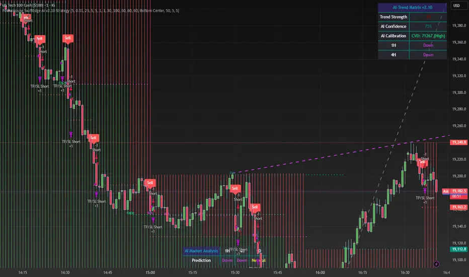
PowerHouse SwiftEdge AI v2.10 StrategyOverview
The PowerHouse SwiftEdge AI v2.10 Strategy is a sophisticated trading system designed to identify high-probability trade setups in forex, stocks, and cryptocurrencies. By combining multi-timeframe trend analysis, momentum signals, volume confirmation, and smart money concepts (Change of Character and Break of Structure ), this strategy offers traders a robust tool to capitalize on market trends while minimizing false signals. The strategy’s unique “AI” component analyzes trends across multiple timeframes to provide a clear, actionable dashboard, making it accessible for both novice and experienced traders. The strategy is fully customizable, allowing users to tailor its filters to their trading style.
What It Does
This strategy generates Buy and Sell signals based on a confluence of technical indicators and smart money concepts. It uses:
Multi-Timeframe Trend Analysis: Confirms the market’s direction by analyzing trends on the 1-hour (60M), 4-hour (240M), and daily (D) timeframes.
Momentum Filter: Ensures trades align with strong price movements to avoid choppy markets.
Volume Filter: Validates signals with above-average volume to confirm market participation.
Breakout Filter: Requires price to break key levels for added confirmation.
Smart Money Signals (CHoCH/BOS): Identifies reversals (CHoCH) and trend continuations (BOS) based on pivot points.
AI Trend Dashboard: Summarizes trend strength, confidence, and predictions across timeframes, helping traders make informed decisions without needing to analyze complex data manually.
The strategy also plots dynamic support and resistance trendlines, take-profit (TP) levels, and “Get Ready” signals to alert users of potential setups before they fully develop. Trades are executed with predefined take-profit and stop-loss levels for disciplined risk management.
How It Works
The strategy integrates multiple components to create a cohesive trading system:
Multi-Timeframe Trend Analysis:
The strategy evaluates trends on three timeframes (1H, 4H, Daily) using Exponential Moving Averages (EMA) and Volume-Weighted Average Price (VWAP). A trend is considered bullish if the price is above both the EMA and VWAP, bearish if below, or neutral otherwise.
Signals are only generated when the trend on the user-selected higher timeframe aligns with the trade direction (e.g., Buy signals require a bullish higher timeframe trend). This reduces noise and ensures trades follow the broader market context.
Momentum Filter:
Measures the percentage price change between consecutive bars and compares it to a volatility-adjusted threshold (based on the Average True Range ). This ensures trades are taken only during significant price movements, filtering out low-momentum conditions.
Volume Filter (Optional):
Checks if the current volume exceeds a long-term average and shows positive short-term volume change. This confirms strong market participation, reducing the risk of false breakouts.
Breakout Filter (Optional):
Requires the price to break above (for Buy) or below (for Sell) recent highs/lows, ensuring the signal aligns with a structural shift in the market.
Smart Money Concepts (CHoCH/BOS):
Change of Character (CHoCH): Detects potential reversals when the price crosses under a recent pivot high (for Sell) or over a recent pivot low (for Buy) with a bearish or bullish candle, respectively.
Break of Structure (BOS): Confirms trend continuations when the price breaks below a recent pivot low (for Sell) or above a recent pivot high (for Buy) with strong momentum.
These signals are plotted as horizontal lines with labels, making it easy to visualize key levels.
AI Trend Dashboard:
Combines trend direction, momentum, and volatility (ATR) across timeframes to calculate a trend score. Scores above 0.5 indicate an “Up” trend, below -0.5 indicate a “Down” trend, and otherwise “Neutral.”
Displays a table summarizing trend strength (as a percentage), AI confidence (based on trend alignment), and Cumulative Volume Delta (CVD) for market context.
A second table (optional) shows trend predictions for 1H, 4H, and Daily timeframes, helping traders anticipate future market direction.
Dynamic Trendlines:
Plots support and resistance lines based on recent swing lows and highs within user-defined periods (shortTrendPeriod, longTrendPeriod). These lines adapt to market conditions and are colored based on trend strength.
Why This Combination?
The PowerHouse SwiftEdge AI v2.10 Strategy is original because it seamlessly integrates traditional technical analysis (EMA, VWAP, ATR, volume) with smart money concepts (CHoCH, BOS) and a proprietary AI-driven trend analysis. Unlike standalone indicators, this strategy:
Reduces False Signals: By requiring confluence across trend, momentum, volume, and breakout filters, it minimizes trades in choppy or low-conviction markets.
Adapts to Market Context: The ATR-based momentum threshold adjusts dynamically to volatility, ensuring signals remain relevant in both trending and ranging markets.
Simplifies Decision-Making: The AI dashboard distills complex multi-timeframe data into a user-friendly table, eliminating the need for manual analysis.
Leverages Smart Money: CHoCH and BOS signals capture institutional price action patterns, giving traders an edge in identifying reversals and continuations.
The combination of these components creates a balanced system that aligns short-term trade entries with longer-term market trends, offering a unique blend of precision, adaptability, and clarity.
How to Use
Add to Chart:
Apply the strategy to your TradingView chart on a liquid symbol (e.g., EURUSD, BTCUSD, AAPL) with a timeframe of 60 minutes or lower (e.g., 15M, 60M).
Configure Inputs:
Pivot Length: Adjust the number of bars (default: 5) to detect pivot highs/lows for CHoCH/BOS signals. Higher values reduce noise but may delay signals.
Momentum Threshold: Set the base percentage (default: 0.01%) for momentum confirmation. Increase for stricter signals.
Take Profit/Stop Loss: Define TP and SL in points (default: 10 each) for risk management.
Higher/Lower Timeframe: Choose timeframes (60M, 240M, D) for trend filtering. Ensure the chart timeframe is lower than or equal to the higher timeframe.
Filters: Enable/disable momentum, volume, or breakout filters to suit your trading style.
Trend Periods: Set shortTrendPeriod (default: 30) and longTrendPeriod (default: 100) for trendline plotting. Keep below 2000 to avoid buffer errors.
AI Dashboard: Toggle Enable AI Market Analysis to show/hide the prediction table and adjust its position.
Interpret Signals:
Buy/Sell Labels: Green "Buy" or red "Sell" labels indicate trade entries with predefined TP/SL levels plotted.
Get Ready Signals: Yellow "Get Ready BUY" or orange "Get Ready SELL" labels warn of potential setups.
CHoCH/BOS Lines: Aqua (CHoCH Sell), lime (CHoCH Buy), fuchsia (BOS Sell), or teal (BOS Buy) lines mark key levels.
Trendlines: Green/lime (support) or fuchsia/purple (resistance) dashed lines show dynamic support/resistance.
AI Dashboard: Check the top-right table for trend strength, confidence, and CVD. The optional bottom table shows trend predictions (Up, Down, Neutral).
Backtest and Trade:
Use TradingView’s Strategy Tester to evaluate performance. Adjust TP/SL and filters based on results.
Trade manually based on signals or automate with TradingView alerts (set alerts for Buy/Sell labels).
Originality and Value
The PowerHouse SwiftEdge AI v2.10 Strategy stands out by combining multi-timeframe analysis, smart money concepts, and an AI-driven dashboard into a single, user-friendly system. Its adaptive momentum threshold, robust filtering, and clear visualizations empower traders to make confident decisions without needing advanced technical knowledge. Whether you’re a day trader or swing trader, this strategy provides a versatile, data-driven approach to navigating dynamic markets.
Important Notes:
Risk Management: Always use appropriate position sizing and risk management, as the strategy’s TP/SL levels are customizable.
Symbol Compatibility: Test on liquid symbols with sufficient historical data (at least 2000 bars) to avoid buffer errors.
Performance: Backtest thoroughly to optimize settings for your market and timeframe.
BTC Daily DCA CalculatorThe BTC Daily DCA Calculator is an indicator that calculates how much Bitcoin (BTC) you would own today by investing a fixed dollar amount daily (Dollar-Cost Averaging) over a user-defined period. Simply input your start date, end date, and daily investment amount, and the indicator will display a table on the last candle showing your total BTC, total invested, portfolio value, and unrealized yield (in USD and percentage).
Features
Customizable Inputs: Set the start date, end date, and daily dollar amount to simulate your DCA strategy.
Results Table: Displays on the last candle (top-right of the chart) with:
Total BTC: The accumulated Bitcoin from daily purchases.
Total Invested ($): The total dollars invested.
Portfolio Value ($): The current value of your BTC holdings.
Unrealized Yield ($): Your profit/loss in USD.
Unrealized Yield (%): Your profit/loss as a percentage.
Visual Markers: Green triangles below the chart mark each daily investment.
Overlay on Chart: The table and markers appear directly on the BTCUSD price chart for easy reference.
Daily Timeframe: Designed for Daily (1D) charts to ensure accurate calculations.
How to Use
Add the Indicator: Apply the indicator to a BTCUSD chart (e.g., Coinbase:BTCUSD, Binance:BTCUSDT).
Set Daily Timeframe: Ensure your chart is on the Daily (1D) timeframe, or the script will display an error.
Configure Inputs: Open the indicator’s Settings > Inputs tab and set:
Start Date: When to begin the DCA strategy (e.g., 2024-01-01).
End Date: When to end the strategy (e.g., 2025-04-27 or earlier).
Daily Investment ($): The fixed dollar amount to invest daily (e.g., $100).
View Results: Scroll to the last candle in your date range to see the results table in the top-right corner of the chart. Green triangles below the bars indicate investment days.
Settings
Start Date: Choose the start date for your DCA strategy (default: 2024-01-01).
End Date: Choose the end date (default: 2025-04-27). Must be after the start date and within available chart data.
Daily Investment ($): Set the daily investment amount (default: $100). Minimum is $0.01.
Notes
Timeframe: The indicator requires a Daily (1D) chart. Other timeframes will trigger an error.
Data: Ensure your BTCUSD chart has historical data for the selected date range. Use reliable pairs like Coinbase:BTCUSD or Binance:BTCUSDT.
Limitations: Does not account for trading fees or slippage. Future dates (beyond the current date) will not display results.
Performance: Works best with historical data. Free TradingView accounts may have limited historical data; consider premium for longer ranges.

TASC 2025.05 Trading The Channel█ OVERVIEW
This script implements channel-based trading strategies based on the concepts explained by Perry J. Kaufman in the article "A Test Of Three Approaches: Trading The Channel" from the May 2025 edition of TASC's Traders' Tips . The script explores three distinct trading methods for equities and futures using information from a linear regression channel. Each rule set corresponds to different market behaviors, offering flexibility for trend-following, breakout, and mean-reversion trading styles.
█ CONCEPTS
Linear regression
Linear regression is a model that estimates the relationship between a dependent variable and one or more independent variables by fitting a straight line to the observed data. In the context of financial time series, traders often use linear regression to estimate trends in price movements over time.
The slope of the linear regression line indicates the strength and direction of the price trend. For example, a larger positive slope indicates a stronger upward trend, and a larger negative slope indicates the opposite. Traders can look for shifts in the direction of a linear regression slope to identify potential trend trading signals, and they can analyze the magnitude of the slope to support trading decisions.
One caveat to linear regression is that most financial time series data does not follow a straight line, meaning a regression line cannot perfectly describe the relationships between values. Prices typically fluctuate around a regression line to some degree. As such, analysts often project ranges above and below regression lines, creating channels to model the expected extent of the data's variability. This strategy constructs a channel based on the method used in Kaufman's article. It measures the maximum distances from points on the linear regression line to historical price values, then adds those distances and the current slope to the regression points.
Depending on the trading style, traders might look for prices to move outside an established channel for breakout signals, or they might look for price action to reach extremes within the channel for potential mean reversion opportunities.
█ STRATEGY CALCULATIONS
Primary trade rules
This strategy implements three distinct sets of rules for trend, breakout, and mean-reversion trades based on the methods Kaufman describes in his article:
Trade the trend (Rule 1) : Open new positions when the sign of the slope changes, indicating a potential trend reversal. Close short trades and enter a long trade when the slope changes from negative to positive, and do the opposite when the slope changes from positive to negative.
Trade channel breakouts (Rule 2) : Open new positions when prices cross outside the linear regression channel for the current sample. Close short trades and enter a long trade when the price moves above the channel, and do the opposite when the price moves below the channel.
Trade within the channel (Rule 3) : Open new positions based on price values within the channel's range. Close short trades and enter a long trade when the price is near the channel's low, within a specified percentage of the channel's range, and do the opposite when the price is near the channel's high. With this rule, users can also filter the trades based on the channel's slope. When the filter is active, long positions are allowed only when the slope is positive, and short positions are allowed only when it is negative.
Position sizing
Kaufman's strategy uses specific trade sizes for equities and futures markets:
For an equities symbol, the number of shares traded is $10,000 divided by the current price.
For a futures symbol, the number of contracts traded is based on a volatility-adjusted formula that divides $25,000 by the product of the 20-bar average true range and the instrument's point value.
By default, this script automatically uses these sizes for its trade simulation on equities and futures symbols and does not simulate trading on other symbols. However, users can control position sizes from the "Settings/Properties" tab and enable trade simulation on other symbol types by selecting the "Manual" option in the script's "Position sizing" input.
Stop-loss
This strategy includes the option to place an accompanying stop-loss order for each trade, which users can enable from the "SL %" input in the "Settings/Inputs" tab. When enabled, the strategy places a stop-loss order at a specified percentage distance from the closing price where the entry order occurs, allowing users to compare how the strategy performs with added loss protection.
█ USAGE
This strategy adapts its display logic for the three trading approaches based on the rule selected in the "Trade rule" input:
For all rules, the script plots the linear regression slope in a separate pane. The plot is color-coded to indicate whether the current slope is positive or negative.
When the selected rule is "Trade the trend", the script plots triangles in the separate pane to indicate when the slope's direction changes from positive to negative or vice versa. Additionally, it plots a color-coded SMA on the main chart pane, allowing visual comparison of the slope to directional changes in a moving average.
When the rule is "Trade channel breakouts" or "Trade within the channel", the script draws the current period's linear regression channel on the main chart pane, and it plots bands representing the history of the channel values from the specified start time onward.
When the rule is "Trade within the channel", the script plots overbought and oversold zones between the bands based on a user-specified percentage of the channel range to indicate the value ranges where new trades are allowed.
Users can customize the strategy's calculations with the following additional inputs in the "Settings/Inputs" tab:
Start date : Sets the date and time when the strategy begins simulating trades. The script marks the specified point on the chart with a gray vertical line. The plots for rules 2 and 3 display the bands and trading zones from this point onward.
Period : Specifies the number of bars in the linear regression channel calculation. The default is 40.
Linreg source : Specifies the source series from which to calculate the linear regression values. The default is "close".
Range source : Specifies whether the script uses the distances from the linear regression line to closing prices or high and low prices to determine the channel's upper and lower ranges for rules 2 and 3. The default is "close".
Zone % : The percentage of the channel's overall range to use for trading zones with rule 3. The default is 20, meaning the width of the upper and lower zones is 20% of the range.
SL% : If the checkbox is selected, the strategy adds a stop-loss to each trade at the specified percentage distance away from the closing price where the entry order occurs. The checkbox is deselected by default, and the default percentage value is 5.
Position sizing : Determines whether the strategy uses Kaufman's predefined trade sizes ("Auto") or allows user-defined sizes from the "Settings/Properties" tab ("Manual"). The default is "Auto".
Long trades only : If selected, the strategy does not allow short positions. It is deselected by default.
Trend filter : If selected, the strategy filters positions for rule 3 based on the linear regression slope, allowing long positions only when the slope is positive and short positions only when the slope is negative. It is deselected by default.
NOTE: Because of this strategy's trading rules, the simulated results for a specific symbol or channel configuration might have significantly fewer than 100 trades. For meaningful results, we recommend adjusting the start date and other parameters to achieve a reasonable number of closed trades for analysis.
Additionally, this strategy does not specify commission and slippage amounts by default, because these values can vary across market types. Therefore, we recommend setting realistic values for these properties in the "Cost simulation" section of the "Settings/Properties" tab.
